How I arrived at the sphere model equation

So, how did I arrive at the sphere model equation describing the forces between two uniformly moving point charges as measured by co-moving spring balances? I started from Coulomb's law of electrostatics:

      (1)

The law describes the force between two stationary charges q₁ and q₂ separated by the distance r. We know from classical electromagnetism and special relativity that the forces between two charges q₁ and q₂ moving at constant velocities u and v, as measured by co-moving spring balances, look rather different from this: they depend on those velocities, the distance between the charges and the speed of light in a rather complicated way. Classical electromagnetism describes the force exerted by q₁ on q₂ in this more general case by means of two fields: the electric field E associated with q₁ and the magnetic field B associated with q₁. These need to be inserted into the Lorentz force law

    (2)

and a relativistic force transformation needs to be applied to obtain the force on q₂ as measured by a co-moving spring balance. I was convinced, however, that it should be possible to explain the forces between moving charges as measured by co-moving spring balances much more simply, in terms of a single 'electric' field surrounding any charge in any state of motion. The first question I needed to answer was what shape this single 'electric' field might take.

Step 1

I assumed that in any point in space and time there is a uniformly moving frame of reference S in which the electric field of any charge at rest - i.e. the electric properties of the space surrounding such a charge - is isotropic (the same in every direction). To me that meant that the field can be represented as a succession of concentric and equally spaced sphere surfaces. In S, any electric field disturbances resulting from the acceleration of a charge at rest would thus propagate in isotropic conditions. It would therefore be possible to synchronize clocks at rest in S using Einstein's clock adjustment procedure, and as a result the speed c at which electric disturbances propagate in S would be the same in every direction.

Note that this set of assumptions is much weaker than those made in classical theory, where it is somewhat implausibly assumed that the electric properties of the space surrounding charges at rest are isotropic in any uniformly moving frame of reference. What is more, in the sphere model there is no need to accept the constancy of the two-way speed of light in every uniformly moving frame of reference as a fundamental law of nature that cannot be explained any further, as is done in classical theory.

With all this in place, it was clear that accelerating a charge from rest in S to a particular velocity u would distort the sphere surface configuration surrounding it as follows:

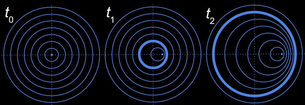
Fig. 1

The sphere fields of two charges q₁ and q₂ travelling at constant velocities u and v in S and separated by the distance r can consequently be represented as follows:

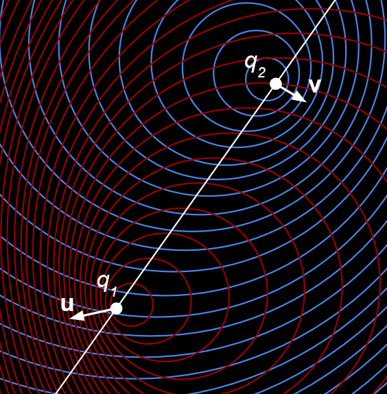
Fig. 2

My hypothesis was now the following: the past accelerations of any two charges q₁ and q₂ moving at u and v in S bring about changes in the sphere field configuration surrounding the charges, and corresponding changes in the flow of information between them, which result in changes in the forces between those charges, as measured by co-moving spring balances, compared to the static case. More specifically, I hypothesised that it should be possible to describe those changes in the sphere field configuration, and corresponding changes in the flow of information, by a series of sphere field parameters x₁, x₂, x₃… and a direction vector y so that (1) would become

    (3)

Let me pause here for a moment to reflect on the significance of this hypothesis: if true, it would mean that the forces between uniformly moving charges as measured by co-moving spring balances could be explained with reference to a single field, the 'sphere field', and without the need to perform any relativistic transformation. The sphere model would thus be able to explain the mysterious appearance of 'magnetic forces' in classical theory. What is more, given the distortions in the sphere fields of charges moving in S, it would imply that locally Einstein clock adjustment would synchronize clocks only in S and not in any other uniformly moving frame of reference. This would instantly put paid to some rather outlandish ideas that are floating around in the literature based on misinterpretations of special relativity, such as the idea that we live in a 'block universe'. As if that wasn't enough, the sphere model would explain how the electric forces between moving charges are transformed in a manner that is consistent with length contraction. It would thus provide a partial explanation of length contraction.

But how might I be able to confirm my hypothesis? I decided to pursue a two-pronged approach.

Step 2

I assumed that the classical results for the forces between uniformly moving charges as measured by co-moving spring balances are empirically correct. This enabled me to work out what I had to aim for in my search for the sphere model parameters  x₁, x₂, x₃… and the direction vector y. For simplicity, I decided to define a cartesian coordinate system in which the charge q₂ is located at the origin and moves in the direction of the x-axis, while the charge q₁ is located in the xy-plane, as follows:

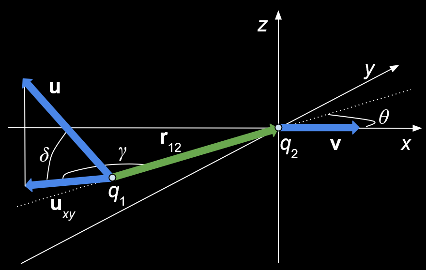
Fig. 3

It is also convenient to define an additional angle α as follows:

This is not an independent parameter and the following relationship holds:

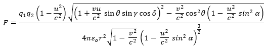
In terms of this coordinate system, using the formulae for the electric and magnetic fields of moving point charges, the Lorentz force law, and the transformations of special relativity, classical theory tells us that the magnitude of the force exerted by q₁ on q₂ as measured by a co-moving spring balance is as follows:

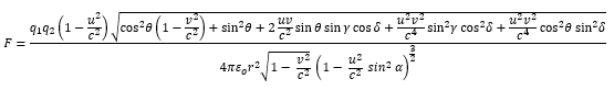
(4)

And the direction of that force as seen from S (i.e. the direction in which q₂ is accelerated in S) is parallel to the vector

     (5)

The task of finding sphere model parameters that would produce this magnitude and this direction seemed formidable. One of the difficulties I saw was that the magnitude was not particularly factorised. Specifically, I saw little hope of finding a single sphere model factor corresponding to the square root term in (4). The first thing I did, therefore, was to play around a bit with (4). I soon found that it could be expressed as follows:

(6)

This looked much more promising. Note how there are now several terms in the equation which are of the form a² - b². This factorises nicely into (a + b)(a - b). My task now looked a little bit more manageable but still quite daunting. How should I go about finding sphere model parameters that would produce (5) and (6)?

Step 3

I started by simply having a look to see which aspects of the sphere field configuration in Figure 2 were different from the sphere field configuration in the static case. The first that struck me was the q₁ sphere surface density along the line connecting the charges. This was clearly different from the density that pertains in the static case (whatever precisely the magnitude of that density might be).

I had soon gathered a few pertinent results: a) the q₁ sphere surface density along the line connecting the charges is constant on the 'near side' of q₁ (the side on which q₂ is located) and on the 'far side' of q₁ (the side on which q₂ is not located); b) as can be seen in Figure 4, information that travels from q₁ to q₂ from the location of q₁ at the 'retarded time' (t₀ in Figure 4), such that it arrives at q₂ at the 'current time' (t₁ in Figure 4), travels through the q₁ sphere field along the line connecting the charges at the current time, in other words the sphere surface densities along that line in its current position are potentially relevant bits of information transmitted from q₁ to q₂; c) if I define the 'density factors' as the factors by which these densities are different from the density in the static case, and if I multiply the near- and far-side density factors, then I obtain one of the terms in (6), namely (1 - u²/c²). It looked like I had found my first sphere model parameter x₁!

Fig. 4

A second parameter was soon to follow: I noticed that the angle at which the connecting line cuts through neighbouring q₁ sphere surfaces is different from the 90-degree angle in the static case, and consequently the path taken by electric information from one sphere surface to the next is longer than the local perpendicular distance between the sphere surfaces. The factor by which it is longer is the same on the near side and the far side. The product of the two turned out to be another factor in (6), namely 1/(1 - u²sin² α/c²).

But the hard bit was yet to come. It was the remaining square root term in (6). It did not seem likely that just taking a long hard look at the sphere field configuration in Figure 2 would enable me to detect that factor in that configuration. I suspected that the square root term had something to do with the frequency at which electric information coming from q₁ arrives at q₂. That frequency could be expected to depend on both u and v. I started to experiment with a number of sphere model frequency factors, initially for special cases and in two dimensions only. It was only when it occurred to me that I might have to look at 'near-side' and 'far-side' frequencies that I was able to make decisive progress. Eventually I discovered that I had to form the geometric mean of near-side and far-side information transmission rates, which depend on the q₁ and q₂ sphere surface configurations, to obtain the desired term.

It thus turned out that each of the factors I had identified - the density factor, the angle factor and the frequency factor - could be regarded as the geometric mean of near-side and far-side density, angle and frequency factors. Is that plausible? In principle I think it is: it seems plausible that the information that is transmitted from q₁ to q₂ concerns a whole area around the mathematical point on which q₁ is centred. That information will have travelled along the line connecting the two charges, so again it is plausible that it includes near-side and far-side information on parameters along that line. The fact that what matters is the geometric mean of near- and far-side factors, rather than some other kind of combination of the two, is perhaps less immediately plausible. No doubt one day somebody will find an explanation for it.

At this point I felt like celebrating. I had succeeded in identifying just three simple sphere field parameters by which (1) had to be modified to obtain the magnitude of the force between two charges moving uniformly in S. But then I remembered that I had not finished the job. I had yet to explain, in terms of the sphere model, why the direction of the force as seen from S is parallel to (5)!

Step 4

Again, the task of obtaining the correct direction vector looked daunting, but this time I succeeded more quickly than I had anticipated. I had a good idea where to look: it would be plausible for the direction vector to depend on the direction from which q₁ information arrives  at q₂. However, when I calculated the 'near-side direction vector' n₁^< (see Figure 5), which describes that direction in S, it wasn't parallel to (5). The near-side direction vector is the vector pointing from the 'retarded' position of q₁ at the centre of the q₁ sphere surface on which q₂ is located to the current position of q₂. I then figured that perhaps I had to include the 'far-side direction vector' n₁^>, in other words the vector pointing from the retarded position of q₁ to the far-side intersection of the line connecting q₁ and q₂ at the current time with the q₁ sphere surface centred on the retarded position. Still that didn't work.

Fig. 5

It was only when I started to look at the situation from the point of view of q₂ that I struck gold. I found that I had to consider the near-side and far-side directions from which q₁ information arrives at q₂ from the point of view of q₂. Those two directions are given by n₁^< - v/c and n₁^> - v/c. Simply adding up those two vectors still didn't do the trick, however. I found that I had to modulate those two vectors by particular factors. Just by looking at the x- and y-components, I was able to calculate the factors that are required to obtain the correct result. They turned out to be q₂ sphere field parameters that I had previously worked out for q₁: the q₂ angle factors! What is more: the z-component worked with those same factors. This could be no accident! I felt vindicated. My intuition had been right. All aspects of the forces between uniformly moving charges as measured by co-moving spring balances could be expressed simply in terms of a few basic sphere model parameters. The end result was as follows:

     (7)

Here d₁, e₁ and f₁ are the q₁ density, angle and frequency factors, and e₂^< and e₂^> are the near- and far-side q₂ angle factors.

To my mind, this is an amazing result. It means that the forces between uniformly moving charges as measured by co-moving spring balances can be expressed simply in terms of a few sphere model parameters, without reference to any 'magnetic field' and without the need to perform any relativistic transformations. Equation (7) can also be written purely in terms of u, v, n₁^< and n₁^>, as follows:

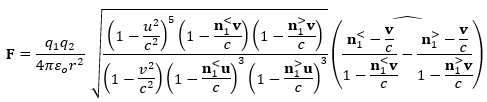      (8)

However, equation (7) shows more clearly how this force comes about, namely as a result of changes in the sphere field configuration compared to the static case described by Coulomb's law. And that concludes my account of how I arrived at the sphere model equation describing the forces between two uniformly moving point charges as measured by co-moving spring balances.

One last thing. The need to systematically take into account near- and far-side sphere field properties is a remarkable feature of the sphere model. I have tried to explain it by assuming that information travelling from q₁ to q₂ in the direction of n₁^< includes full information on near- and far-side sphere field properties along the line connecting the two charges at the current time. There is another possibility. It is that in S the information travels well and truly in the near- and far-side directions given by  n₁^< and n₁^> and is exchanged instantly over the q₁ sphere surface on which q₂ is located at the current time, t₁, as shown in Figure 6 below.

Fig.6

The idea would be that, while energy in the form of sphere field disturbances can only be transmitted at c in S, since it has to travel outwards from one sphere surface to the next, information on interlinked near- and far-side sphere field properties can be exchanged instantly on one and the same sphere surface. The whole situation reminds me a bit of what I've read here and there about the phenomenon of quantum entanglement. I am no expert on quantum mechanics, so I don't know whether there is a connection. But it is intriguing to think that, in addition to solving the mystery of the magnetic field in classical electrodynamics, the sphere model might also shed some new light on quantum entanglement, or vice versa.