If a long time has passed since my last blog post, it's not because I've lost interest in quantum mechanics. It's because I've been distracted by my sphere model of electricity, first introduced here, here and here.
After months of working on it whenever I could snatch a few minutes in between more important things, I have found relatively simple and plausible mathematical expressions for the forces between point charges moving at constant velocities, using nothing but a few basic sphere model parameters and without any recourse to special relativity or magnetism.
To be more specific: Let two charges q1 and q2, separated by the vector r, move at constant velocities u and v in an inertial frame of reference Σ in which electric effects propagate in symmetrical conditions in all directions and clocks have been Einstein-adjusted.
Then the magnitude of the force on q2 as measured by a co-moving Newton meter (or spring balance) can be written as
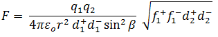 (1)
(1)
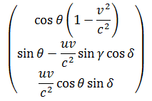
and the direction of the force in Σ (i.e. the direction of the Newton meter in Σ) is parallel to the vector
 (2)
(2)
where
and
At the heart of this approach lies the idea that the information about q1 that acts on q2 is 'complete' in the sense that it includes parameters such as sphere density and frequency factors from either side of q1 (the 'leading' side and the 'trailing' side), along the line connecting q1 and q2.
To compare my results with those obtained in classical electromagnetism, for any u, v and r a cartesian coordinate system can be chosen such that v starts in the origin and points in the direction of the x-axis, and r lies in the xy-plane:
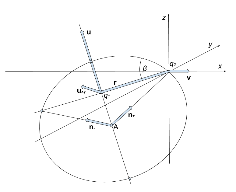
The point A is at the centre of the electric sphere associated with q1 whose surface includes q2. The cross-section of the sphere shown in the figure lies in the plane defined by u and r. Dots indicate locations where lines meet or intersect.
In terms of this coordinate system, r, u and v can be specified by their magnitudes r, u and v, the angle θ between r and v, and the following two angles:
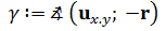
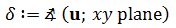 where ux,y is the projection of u onto the xy-plane. In addition, we can define
and
Using nothing but elementary geometry, d, f and n can then be expressed as follows:
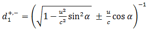 (3)
(3)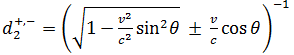 (4)
(4)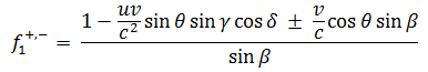 (5)
(5)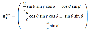 . (6)
. (6)
The angles α and β have been introduced for convenience only. They are not independent parameters and the following relationships hold:
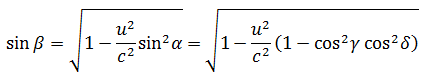 (7)
(7)
Inserting (3), (4), (5) and (6) into (1) and (2), it turns out that the magnitude of the force on q2 as measured by a co-moving Newton meter, as well as the direction of that force (the direction of the Newton meter) in Σ, are the same in my sphere model of electricity as they are in classical electromagnetism. According to my calculations, in terms of the coordinates defined above this magnitude is:
 (8)
(8)
(8)
and the direction is:
 (9)
(9)
Et voilà!
So, what is the significance of these results?
I think it's twofold. First, my results suggest that it may be possible to develop a model of electricity in which the forces between moving charges can be expressed in much simpler and more plausible terms than in classical electromagnetism.
Second, and more importantly from my point of view, my results suggest that there may be a simple cause for a hitherto unexplained and rather mysterious empirical fact at the heart of special relativity: the length contraction of moving objects in inertial frames of reference in which clocks have been Einstein-adjusted. This is because 'electric length contraction' – the transformation of the forces between moving charges in a way that is consistent with length contraction – follows from the formulas for the forces between moving charges.
The fact that electric field disturbances always travel in tandem (the 'no overtaking rule') follows directly from the sphere model of electricity. Together with length contraction, it implies time dilation, at least as measured by light clocks. From length contraction and time dilation, the whole apparatus of special relativity follows. The sphere model of electricity can thus potentially help to achieve a deeper understanding of special relativity. Which is my ultimate goal in this blog.
But how are your results simple? They look much more complicated than the F = q(E + vxB) formula in classical electromagnetism!
It's true that this classical equation is a nice and simple formula. But in classical electromagnetism, the devil lies in determining E and B, even in situations as simple as that of a moving point charge. Textbooks on classical electromagnetism typically get to the point of deriving the electric and magnetic fields of point charges moving at constant velocities only after many pages of developing the theory, using a range of advanced mathematical techniques.
What is more, F = q(E + vxB) cannot be used directly to determine the force on q2 as measured by a co-moving Newton meter. To achieve that, the additional step of a relativistic force transformation is required. Nor does F = q(E + vxB) give the direction of that force (i.e. the direction of the Newton meter) in Σ. It's really just a theoretical quantity which first has to be translated into observables by means of additional calculations. And the same can be said of E and B.
The sphere model of electricity, on the other hand, can be developed on a few pages from Coulomb's law for stationary charges to the point of explaining the forces between two moving charges using nothing but basic high-school-level geometry.
Supposing your sphere model is indeed relatively simple (though at first sight it doesn't necessarily look like that), in what sense is it more plausible than classical theories?
I'd argue that it does not take much for a model of electricity that encompasses magnetic phenomena to be more plausible than classical electromagnetism. The reason is that classical electromagnetism has no intrinsic plausibility at all. Nor does it make any claim to plausibility. It just happens to work. Indeed, it works very well. But nobody knows why.
For example, nobody knows how magnetic field effects come about, at least not in terms of classical electromagnetism alone. This is so even though magnetic field laws involve nothing but electric parameters and the speed of light, so they should be a consequence of electric laws plus the fact that electric field disturbances propagate at c.
While in classical electromagnetism magnetic effects are an ad hoc, unexplained add-on, they can be regarded, and are sometimes described, as a consequence of special relativity. However, the length contraction formula in special relativity, which plays a role in these explanations, also involves the speed at which electric effects propagate, so length contraction should be a consequence of the fact that electric field disturbances (and perhaps all force field disturbances) propagate at c in inertial frames of reference in which clocks have been Einstein-adjusted. But special relativity provides no explanation of length contraction (unless the constancy of the two-way speed of light for all observers is taken as the equally implausible and unexplained starting point).
The sphere model of electricity, on the other hand, points to a relatively plausible explanation of the forces between moving charges in frames of reference in which electric field disturbances travel in symmetric conditions in all directions and clocks have been Einstein adjusted, without using the concept of the magnetic field or length contraction. As a result, the sphere model of electricity provides a relatively plausible explanation of 'electric length contraction' and of at least some phenomena traditionally described in terms of magnetic fields.
I realise that I will have to explain in more detail what I mean by 'relatively plausible explanation'. What I can say for sure is that I have found relatively simple mathematical expressions for the forces between point charges moving at constant velocities using nothing but a few basic sphere model parameters. Admittedly, I had the benefit of hindsight: it was only the prior knowledge of the forces between moving charges that enabled me to ascertain whether those forces take a simple and plausible form in the sphere model of electricity!
I also believe that it is plausible that the sphere model parameters presented in this blog post should play a role in determining the forces between moving charges. For example, as can be seen in (2), in the sphere model of electricity the direction of the force on q2 in Σ is a simple linear combination of two vectors which can be understood as representing the flow of information from q1 to q2.
More detailed explanations will have to wait until future blog posts. Perhaps a whole series of posts devoted exclusively to a careful development of the sphere model of electricity.
Before I get on with that, I will have to check and double-check all my calculations, including all those pesky plus and minus signs; sift through the literature to make sure it hasn't all been done before; and gather my thoughts on the significance and correct interpretation of my findings.