Are we on the brink of a revolution in our understanding of electrodynamics?

Do you often lie awake late at night worrying about the origin of magnetic forces between moving charges or the reason for the constancy of the two-way speed of light for any observer?

If you do, then the sphere model of electricity, accessible in full here and explained in simplified form here, is for you.

That's because the model sheds a good deal of light on the following questions:

• how magnetic effects between moving charges come about
• why the speed of light is independent from the speed of the source
• why moving bodies are length-contracted by the relativistic factor for any observer using Einstein-adjusted clocks
• why moving clocks run slow by the relativistic factor for any observer using Einstein-adjusted clocks
• why the two-way speed of light is constant for every observer
• why the one-way speed of light is constant for every observer using Einstein-adjusted clocks
• in which conditions Einstein's clock adjustment procedure synchronizes distant clocks
• what follows from all this for the correct interpretation of special relativity.

If you never lie awake late at night worrying about those questions, then now may be a good time to start doing so.

For the sphere model has the potential to radically overhaul our understanding of electrodynamics and special relativity.

Let me explain why.

Turn back the clock 150 years or so when the world had not yet heard about special relativity and Maxwell was putting the finishing touches to his theory of electromagnetism.

Magnetic fields were conceived of as vortices in an all-pervasive medium caused by the movement of charged particles. The rotary motions in the medium were thought to deflect other moving charges from their path.

The magnetic forces thus produced were believed to act in a direction perpendicular to the direction of motion of the charges on which they act.

The speed of propagation of electromagnetic disturbances was thought to be a result of the electric and magnetic properties of the hypothetical all-pervasive medium, also known as the aether.

Wind forward 50 years and this picture of the origin of the forces between moving charges was crumbling fast.

It turned out that there was no aether and no rotary motion, and that in general magnetic fields do not deflect charged particles in a direction perpendicular to their direction of motion in the first place.

Special relativity came to the rescue of the faltering theory by stipulating that moving bodies respond differently to transverse and longitudinal forces, to correct for the direction error.

But essentially electromagnetism was now devoid of any physical substance. All that was left of it was a mathematical shell without any explanatory power, propped up by crutches provided by special relativity.

Since then nobody has come up with a convincing alternative, so the theory has limped on from textbook to textbook and from generation to generation.

Let's now shed all this historical baggage for a moment. Let's make a fresh start by pretending we've never heard of magnetic fields or magnetic forces.

Let's pretend that all we know is Coulomb's law of electrostatics, the fact that electric disturbances propagate at c, and the fact that the forces between moving charges (as measured by co-moving spring balances) depend on that propagation speed as well as on the states of motion of those charges (including past states of motion).

How would we then go about explaining this state of affairs?

We could start from a simple assumption that is in line with Coulomb's law and that is much weaker than the assumptions made in classical theory: in every point in space and time there is an inertial frame of reference in which the electric properties surrounding stationary charges are isotropic (the same in every direction).

We could then ask: in such a frame of reference, how are the electric properties and the flow of information between charged particles modified as a result of acceleration to give rise to the forces we observe between moving charges?

This is the question I started to work on eight years ago or so, and it has led me inevitably and inexorably to the sphere model of electricity.

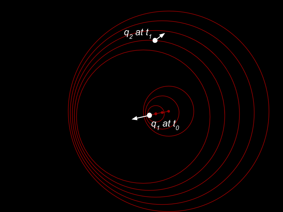
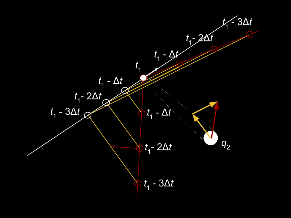
The sphere model is all about the way in which past accelerations modify the sphere arrangements surrounding charged particles and the flow of information between them.

The sphere model not only revolutionizes our understanding of the forces between uniformly moving charges but also sheds new light on special relativity: it implies that, in general, events with equal time coordinates as determined by Einstein-adjusted clocks are not simultaneous.

So, are we on the brink of a revolution in our understanding of electrodynamics?

The answer has to be 'no'.

The sphere model only covers the forces between uniformly moving charges. A fully-fledged model would have to explain the forces between charges in any state of motion.

What is more, the model at best only offers some intangible and difficult-to-understand conceptual advantages over classical electromagnetism. It makes no new predictions (at least not in its current state of development) and it doesn't enable us to build any new machines.

Why would any working physicists want to devote any of their precious time to it?

As for myself, I'm not even a working physicist. I've been working on the sphere model by snatching a few minutes here and there between paid work and family life.

Extending the model to moving charges in any state of motion promises to be mathematically considerably more challenging than developing it for uniformly moving charges.

I'm sure it can be done. All the ingredients are there. But doing it, if indeed I decide to have a go, might well take me another ten years. And I need a break.

The revolution will have to wait a bit longer.

The sphere model of electricity made simple

The most frequent complaint I have had about the sphere model of electricity to date is that it is too complex.

I am therefore presenting it here in really simple terms, in as few words as possible.

All the essential characteristics of the sphere model can be seen in this animation:

The animation shows an electric point charge which is initially at rest and whose electric properties are isotropic (the same in every direction). The particle's electric properties while at rest are represented by equally spaced, concentric sphere surfaces, shown here in cross section.

The particle then gets briefly accelerated to near the speed of light c (about 4/5 c), travels at that speed for a little while (the blue line), gets briefly accelerated/deflected a few more times (in the locations where the dots change colour and direction) and is finally brought to a sudden halt back where it started.

In the sphere model, information on the particle's state of motion is constantly sent out in all directions and always travels from one sphere surface to the next in the same amount of time. This has two important consequences:

1. After acceleration, the sphere field of the particle is no longer isotropic: it is compressed in the direction of movement and stretched out in the opposite direction. However, it becomes isotropic again when the particle is brought back to a halt.
2. Each acceleration/deflection causes a disturbance in the sphere surface arrangement (a change in the sphere surface densities), which radiates outwards at one and the same speed, which in the sphere model is the speed of light, c.

The second point comes out more clearly in a second animation, in which I have speeded up the sequence of events and have highlighted the locations of the sphere surface disturbances. The effect is comparable to a few raindrops falling close to each other on a lake, although the way it comes about is quite different:

It can be seen that the electric disturbances caused by a sudden acceleration/deflection spread out at the same speed in all directions from the location where the acceleration/deflection took place. This is in line with what we know to happen in the real world.

The fact that the sphere model correctly describes the propagation of electric disturbances caused by the acceleration/deflection of charged particles is not surprising because I designed the model that way.

What is perhaps more remarkable is that the model also provides a simple and plausible explanation of the forces between uniformly moving charges as measured by co-moving spring balances.

The sphere model explains such forces in terms of the way in which past accelerations modify the sphere surface arrangements surrounding the charges.

To see how, let's look at a frame from the animation which shows the charge q1 at the current time t1 and in which I've added a second charge q2:

The current location and velocity of q1 are irrelevant for the force on q2 because information about q1 in that location has not yet reached q2. Instead, we need to consider the 'retarded time' t0 when q1 was at the centre of the sphere on which q2 is located:

The effect on q2 would be the same if q1 had continued at a constant velocity until the current time t1, as shown in this diagram:

Imagine for a moment that the line CB is a rod to which the charge q1 is attached. We can then see that the information that left q1 in A at the retarded time travelled through the sphere arrangement along the rod before it reached q2.

The animation below shows how this happens:

The relevant distance r between q1 and q2 is thus the line CB.

We now need to consider the properties of the sphere arrangement locally in C along the line DB, because these are the properties that are communicated to q2.

In the sphere model, the first property that is relevant is the mean sphere density along DB (using the geometric mean) in the vicinity of C. Let's call the factor by which this is different from the sphere density in the static case 'the density factor'. In the sphere model, the distance r = CB needs to be multiplied by the density factor.

The second property that is relevant is the angle at which the line DB cuts through the q1 sphere surfaces. This is different from the 90° angle that applies in the static case. It means that the path between adjacent sphere surfaces along the line DB is longer than the local distance between those sphere surfaces.

Let's call the factor by which it is longer the 'angle factor'. In the sphere model, the distance r = CB must be divided by the angle factor.

So far the only way in which Coulomb's law of electrostatics needs to be modified is thus by using CB as the distance between the charges and multiplying/dividing that distance by the density factor/the angle factor.

But there is another factor which is different from the static case. This concerns the way in which the information which arrives at q2 is communicated to q2.

In the sphere model, the information appears to arrive at q2 from two directions: AD and AB. These two directions are associated with two 'information transmission rates'. The information transmission rates are the periods of time it takes for q1 information along the line DB to traverse the innermost q2 sphere surface.

The information transmission rates depend on the velocity of q2 as well as that of q1.

To see why this is the case, consider the animation below:

Let's call the mean factor (again using the geometric mean) by which the transmission rates are different from the transmission rate in the static case the 'frequency factor'.

In the dynamic case, Coulomb's law needs to be multiplied by the frequency factor.

Coulomb's law, the density factor, the angle factor and the frequency factor are all we need to determine the magnitude of the forces between two charges moving at constant velocities.

As for the direction of the force, in the sphere model it is determined by the two directions AD and AB from which q1 information arrives at q2.

However, from the point of view of q2, the information does not arrive from those two directions but from the directions given by the yellow lines in the illustration below.

To understand why, it's useful again to imagine that q2 is attached to two rods in the directions of the yellow lines in this illustration.

It is then clear that q1 information approaches q2 along those rods.

It turns out that the two directions given by the two sets of parallel yellow lines have to be weighted by the same kind of angle factor introduced above for q1. This time the relevant angle is the angle between AB and AD (the red lines) on the one hand and the directions along which the information arrives at q2 from the point of view of q2 (the yellow lines) on the other.

The red arrow in the illustration above illustrates qualitatively the resulting overall direction of the force on q2 in this particular example.

And that concludes my discussion of the forces between moving charges in the sphere model.

To summarise it all in two sentences:

In the sphere model, to obtain the magnitude of the force between two charges q1 and q2 moving at constant velocities, Coulomb's law must be modified by three factors (the density factor, the angle factor and the frequency factor) which describe the effects of past accelerations on the sphere surface arrangements surrounding the charges and of associated changes in the flow of information from one charge to the other.

The direction of the force exerted by q1 on q2 is a combination of the two directions from which q1 information arrives at q2 from the point of view of q2, modulated by the angle factor for q2.

This is about as simple as I can make it.

The second most frequent complaint I have had about the sphere model is that it is superfluous since we already have a fully functioning theory of the kind of interactions between charged particles considered in the sphere model: classical electromagnetism. So why bother with the sphere model? I will discuss this second complaint in my next blog post.